Outlines

• Unsupervised machine learning
  • \(k\)-means Clustering algorithm
  • Hierarchical Clustering algorithm

Unsupervised machine learning

• Unsupervised machine learning (a.k.a. cluster analysis) is a set of methods to assign objects into clusters when class labels are unknown.

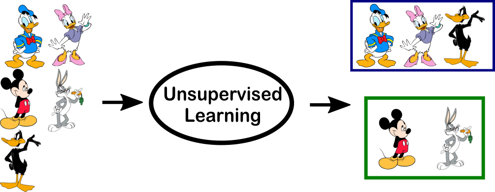
https://cdn-images-1.medium.com/max/1600/1*6hfFWPITJxbtw4ztoC1YeA.png

Motivating example in R

• How to cluster the following data?

library(MASS)
set.seed(32611)
a<- mvrnorm(50, c(0,0), matrix(c(1,0,0,1),2))
b<- mvrnorm(50, c(5,6), matrix(c(1,0,0,1),2))
c<- mvrnorm(50, c(10,10), matrix(c(1,0,0,1),2))
d0 <- rbind(a,b,c)
plot(d0)

Motivating example in R (applying kmeans)

set.seed(32611)
result_km <- kmeans(d0, centers = 3)
plot(d0, col=result_km$cluster)
legend("topleft", legend = 1:3, col = 1:3, pch=1)

\(k\)-means

• Objective function:
  • Minimize the within-cluster dispersion to the cluster centers.
• Pre-specify number of clusters \(K\)

\(k\)-means objective function

\[\min_C \sum_{k=1}^K \sum_{i \in C_k} \|x_i - \bar{x}_{C_k}\|^2,\]

• \(i\) is a sample index.
• \(K\) is total number of clusters.
• \(x_i \in \mathbb{R}^p\) is a \(p\)-dimensional vector.
• \(C_k\) is a collection of samples belong to cluster \(k\)
• \(\bar{x}_{C_K}\) is the cluster center of \(C_K\).
  • \(\bar{x}_{C_k} = \frac{1}{|C_k|} \sum_{i\in C_k} x_i\)
  • \(|C_k|\) is number of samples in cluster \(k\)
• \(C = (C_1, \ldots, C_K)\)

\(k\)-means algorithm

1. Initialize \(K\) centers \(c_1, \ldots, c_K\) as starting values.
2. (Updating clustering labels) Form the clusters \(C_1, \ldots, C_K\) as follows.
   • Denote the clustering labels for subject \(i\): \(g_i = \arg \min_k \|x_i - c_k\|^2\).
   • \(C_k = \{i: g_i = k\}\)
3. (Updating clustering centers) For \(k = 1, \ldots, K\), set the \(k^{th}\) clustering center of \(c_k\) as: \[c_k \rightarrow \frac{1}{|C_k|} \sum_{i\in C_k} x_i\]
4. Repeat 2 and 3 until converge
5. Output: centers \(c_1, \ldots, c_K\) and clusters \(C_1, \ldots, C_K\).

\(k\)-means 2-dimensional example

• example data

set.seed(32611)
N<-100
d1<-mvrnorm(N, c(0,3), matrix(c(2, 1, 1, 2), 2, 2))
d2<-mvrnorm(N, c(-2,-2), matrix(c(2, 1, 1, 2), 2, 2))
d3<-mvrnorm(N, c(2,-2), matrix(c(2, 1, 1, 2), 2, 2))
d <- rbind(d1, d2, d3)
colnames(d) <- c("x", "y")
label <- c(rep("1", N), rep("2", N), rep("3", N))

\(k\)-means demonstration

K <- 3
set.seed(32611)
centers <- mvrnorm(K, mu = c(0,0), Sigma = diag(c(1,1)))
colnames(centers) <- c("x", "y")

plot(d, pch=19)
points(centers, col = 2:4, pch=9, cex=2)

## update group labels
groupsDist <- matrix(0,nrow=nrow(d),ncol=K)
for(k in 1:K){
  vecDiff <- t(d) - centers[k,]
  adist <- apply(vecDiff,2,function(x) sum(x^2))
  groupsDist[,k] <- adist
}
groups <- apply(groupsDist,1,which.min)

plot(d, pch=19, col=groups + 1)
points(centers, pch=9, cex=2)



## update centers
for(k in 1:K){
  asubset <- d[groups==k,]
  centers[k,] <- colMeans(asubset)
}

groups0 <- groups ## save the previous clustering result, in order to test convergence

plot(d, pch=19)
points(centers, col = 2:4, pch=9, cex=2)

Apply kmeans on the iris data example (\(p>2\))

• Visualize by PCA

iris.data <- iris[,1:4]
ir.pca <- prcomp(iris.data,
                 center = TRUE,
                 scale = TRUE) 
PC1 <- ir.pca$x[,"PC1"]
PC2 <- ir.pca$x[,"PC2"]
variance <- ir.pca$sdev^2 / sum(ir.pca$sdev^2)
v1 <- paste0("variance: ",signif(variance[1] * 100,3), "%")
v2 <- paste0("variance: ",signif(variance[2] * 100,3), "%")
plot(PC1, PC2, col=as.numeric(iris$Species),pch=19, xlab=v1, ylab=v2)
legend("topright", legend = levels(iris$Species), col =  unique(iris$Species), pch = 19)

Apply \(k\)-means on the iris data

set.seed(32611) 
kmeans_iris <- kmeans(iris.data, 3)

plot(PC1, PC2, col=as.numeric(kmeans_iris$cluster),pch=19, xlab=v1, ylab=v2)
legend("topright", legend = unique(kmeans_iris$cluster), col =  unique(kmeans_iris$cluster), pch = 19)

Put together (original lables and \(k\)-means labels)

par(mfrow=c(1,2))
plot(PC1, PC2, col=as.numeric(iris$Species),pch=19, xlab=v1, ylab=v2, main="true label")
legend("topright", legend = levels(iris$Species), col =  unique(iris$Species), pch = 19)

plot(PC1, PC2, col=as.numeric(kmeans_iris$cluster),pch=19, xlab=v1, ylab=v2, main="kmeans label")
legend("topright", legend = unique(kmeans_iris$cluster), col =  unique(kmeans_iris$cluster), pch = 19)

Some issues about kmeans algorithm

• Is kmeans a deterministic algorithm? Or random?
• How to determine the optimal K?
• How to compare two sets of clustering results?

Is kmeans deterministic algorithm? Or random?

• original result

set.seed(32611)
result_km <- kmeans(d0, centers = 3)
plot(d0, col=result_km$cluster)
legend("topleft", legend = 1:3, col = 1:3, pch=1)

• label switching

set.seed(32610)
result_km <- kmeans(d0, centers = 3)
plot(d0, col=result_km$cluster)
legend("topleft", legend = 1:3, col = 1:3, pch=1)

• local minimum

set.seed(32619)
result_km <- kmeans(d0, centers = 3)
plot(d0, col=result_km$cluster)
legend("topleft", legend = 1:3, col = 1:3, pch=1)

• can set more number of initialization (e.g., nstart) to try to avoid local minimum problem

kmeans(d0, centers = 3, nstart = 20)

## K-means clustering with 3 clusters of sizes 50, 50, 50
## 
## Cluster means:
##         [,1]        [,2]
## 1  5.0201835  5.84577942
## 2 10.0223462  9.93004155
## 3  0.1262428 -0.05688753
## 
## Clustering vector:
##   [1] 3 3 3 3 3 3 3 3 3 3 3 3 3 3 3 3 3 3 3 3 3 3 3 3 3 3 3 3 3 3 3 3 3 3 3 3 3
##  [38] 3 3 3 3 3 3 3 3 3 3 3 3 3 1 1 1 1 1 1 1 1 1 1 1 1 1 1 1 1 1 1 1 1 1 1 1 1
##  [75] 1 1 1 1 1 1 1 1 1 1 1 1 1 1 1 1 1 1 1 1 1 1 1 1 1 1 2 2 2 2 2 2 2 2 2 2 2
## [112] 2 2 2 2 2 2 2 2 2 2 2 2 2 2 2 2 2 2 2 2 2 2 2 2 2 2 2 2 2 2 2 2 2 2 2 2 2
## [149] 2 2
## 
## Within cluster sum of squares by cluster:
## [1] 99.84741 87.84906 87.79105
##  (between_SS / total_SS =  94.7 %)
## 
## Available components:
## 
## [1] "cluster"      "centers"      "totss"        "withinss"     "tot.withinss"
## [6] "betweenss"    "size"         "iter"         "ifault"

How to determine the optimal K? – Elbow method

• Within sum of squares W(k) is a decreasing function of k.
• Normally look for a turning point of elbow-shape to identify the number of clusters, k.

How to determine the optimal K? – Gap statsitics

• Instead of the above arbitrary criterion, the Gap statsitics proposes to maximize the following Gap statistics.

\[\max Gap_n (k) = \frac{1}{B}(\sum_{b = 1}^B\log(W_b^*(k))) - \log(W(k))\]

• Gap statistics is the difference between observed WCSS and the background.
  • \(W(k)\): within cluster sum of square of the observed data.
  • The background expectation is calculated from random permutation from the original data.
  • \(W_b^*(k)\): within cluster sum of square of the permutated data (bth permutation).

Gap statistics

library(cluster)
gsP.Z <- clusGap(d, FUN = kmeans, K.max = 8, B = 50)
plot(gsP.Z, main = "k = 3  cluster is optimal")

gsP.Z

## Clustering Gap statistic ["clusGap"] from call:
## clusGap(x = d, FUNcluster = kmeans, K.max = 8, B = 50)
## B=50 simulated reference sets, k = 1..8; spaceH0="scaledPCA"
##  --> Number of clusters (method 'firstSEmax', SE.factor=1): 3
##          logW   E.logW       gap     SE.sim
## [1,] 5.769038 6.051298 0.2822604 0.01953592
## [2,] 5.412645 5.742842 0.3301974 0.03763254
## [3,] 5.118928 5.536650 0.4177221 0.02187489
## [4,] 5.031797 5.344077 0.3122792 0.01963785
## [5,] 4.904344 5.234730 0.3303857 0.02161604
## [6,] 4.789622 5.132684 0.3430620 0.02399886
## [7,] 4.779464 5.052895 0.2734309 0.02399082
## [8,] 4.648428 4.975084 0.3266552 0.02359000

How to evaluate the clustering results?

Rand index

• rand index (ranges from 0 to 1):
  • 0: poor agreement
  • 1: perfect agreement

suppressMessages(library(fossil))
set.seed(32611)
g1 <- sample(1:2, size=10, replace=TRUE)
g2 <- sample(1:3, size=10, replace=TRUE)
rand.index(g1, g2)

## [1] 0.4444444

Adjusted Rand index

Adjusted Rand index is the corrected-for-chance version of the Rand index:

\[AdjustedRandIndex = \frac{RI - expected(RI)}{MaxRI-expected(RI)}\]

• Adjusted rand index can be negative:
  • 0: the two clustering assignment are not related
  • 1: perfect agreement

adj.rand.index(g1, g2)

## [1] 0.1697417

Hierarchical Clustering example

set.seed(32611)
index <- sample(nrow(iris), 30)
iris_subset <- iris[index, 1:4]
species_subset <- iris$Species[index]

hc <- hclust(dist(iris_subset))
plot(hc)

Hierarchical Clustering example (with color)

suppressMessages(library(dendextend))
dend = as.dendrogram(hc)
labels_colors(dend) = as.numeric(species_subset)[order.dendrogram(dend)]

plot(dend)
legend("topright", legend=levels(species_subset), col=1:3, pch=1)

\(K\)-means and hierarchical clustering

• \(K\)-means: Partitioning
• hierarchical clustering: Hierarchical

Hierarchical methods

• Hierarchical clustering methods produce a tree or dendrogram.

• No need to specify how many clusters

• The tree can be built in two distinct ways:
  • bottom-up: agglomerative clustering.
  • top-down: divisive clustering.

Hierarchical clustering illustration

• After two data points are merged together, regard it as one single point.
• Height of the tree represents the distance between two points.

Distance between clusters

Distance between clusters

Select a distance measurement \(d\) (e.g. Euclidean distance)

• single linkage \[d(A, B) = \min_{x\in A, y \in B} d(x,y)\]

• average linkage \[d(A, B) = \frac{1}{N_AN_B}\sum_{x\in A, y \in B} d(x,y)\]

• centroid linkage \[d(A, B) = d(\bar{x},\bar{y}),\] where \({x\in A, y \in B}\)

• complete linkage \[d(A, B) = \max_{x\in A, y \in B} d(x,y)\]

Hierarchical tree ordering

• The leafs position can be random.

Hierarchical clustering algorithm

1. Input: dissimilarity matrix (distance matrix \(d \in \mathbb{R}^{n \times n}\))
2. Let \(T_n = \{C_1, C_2, \ldots, C_n\}\).
3. For \(j = n - 1\) to \(1\):
   1. Find \(l,m\) to minimize \(d(C_l, C_m)\) over all \(C_l, C_m \in T_{j+1}\)
   2. Let \(T_j\) be the same as \(T_{j+1}\) except that \(C_l\) and \(C_m\) are replaced with \(C_l \cup C_m\)
4. Return the sets of clusters \(T_1, \ldots, T_n\)

• The result can be represented as a tree, called a dendogram.
• We can then cut the tree at different places to yield any number of clusters.

Cut Hierarchical trees

plot(d0)

hc <- hclust(dist(d0))
plot(hc)

res_cutree <- cutree(hc, k = 1:5) #k = 1 is trivial

set.seed(32611)
result_km <- kmeans(d0, centers = 3)

table(res_cutree[,3], result_km$cluster)

##    
##      1  2  3
##   1 50  0  0
##   2  0 50  0
##   3  0  0 50

rand.index(res_cutree[,3], result_km$cluster)

## [1] 1

adj.rand.index(res_cutree[,3], result_km$cluster)

## [1] 1